Redundancy analysis of an RC circuit using MATLAB

This page demonstrates how to detect redundancy in a circuit model, using the RC circuit as a case study. First the transfer function is derived symbolically using Modified Nodal Analysis (MNA), from which all coefficients containing parameters are extracted. This exhaustive summary is then analysed for redundancy, finding that only one combination of parameters can be estimated.

Complete code is available at the bottom of the page.

Symbolically deriving the transfer function of the RC circuit

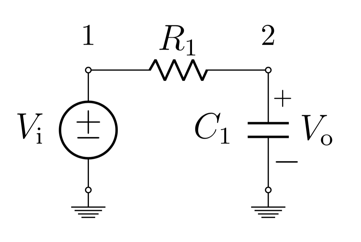Figure 1: Schematic of the RC circuit labelled with nodes.

To detect redundancy in a circuit model, the first step is to define the parameters. For the RC circuit this is R1 and C1, represented in MATLAB using the symbolic type from the Symbolic Toolbox. theta is then a 1xN vector that contains all parameters:

syms R1 C1

theta = [R1 C1];

For this example the transfer function will be used to demonstrate the analysis. To find the transfer function using MNA, first the system matix S must be defined from the components and their topology. The circuit has two nodes, for which each component must be defined as connected positively with a 1, connected negatively with a -1, and not connected with a 0. For passive components like the resistor and capacitor polarity does not matter. For components connected to ground only one non-zero element is needed.

N_R = [1 -1]; % Resistor connected between node 1 and 2
N_C = [0  1]; % Capacitor connected between node 2 and ground
N_V = [1  0]; % Voltage source connected between node 1 and ground
N_O = [0  1]; % Output voltage measured between node 2 and ground

syms s  % Laplace variable

% Conductances
G_R = 1/R1;
G_C = s*C1;

% System matrix
S = [N_R.'*G_R*N_R + N_C.'*G_C*N_C N_V';...
        N_V, 0];

From S the transfer functions of the system can be found by solving for the nodal voltages, performed as a Gauss-Jordan Elimination solve against the voltage input vector.

% Vector containing no current sources and 1 voltage source
U = [0; 0; 1];

% All transfer functions (Vi->Vi, Vi->V2, Vi->Iv)
rcTransfers = S\U;

% H(s) = 1/(1 + s*C1*R1)
ioTransfer = [N_O 0]*rcTransfers;

Extracting the exhaustive summary from the transfer function

Finding the coefficients of the RC i/o transfer function can be done by first separating the transfer function into numerator and denominator, followed by finding the coefficients of s.

[num, den] = numden(ioTransfer);

% Initial exhaustive summary [1 1 C1*R1]
kappaInit = [coeffs(num, s), coeffs(den, s)];

This exhaustive summary is not yet valid as it contains [1 1 C1*R1]. Two of these terms do not contain parameters and therefore should be removed from the vector. Although not needed in this case, should there be repeated elements in the vector they should also be removed to minimise computation time. Both of these operations can be accomplished in a single line using two nested functions

kappa = unique(kappaInit(has(kappaInit, theta)));

unique outputs a vector that contains all of the unique elements of the input vector, i.e. any duplicate entries are removed. has returns a vector of boolean flags that indicate whether that element in the vector contains an element in the second vector. Therefore kappaInit(has(kappaInit, theta)) selects all of the elements of kappaInit that contain parameters in theta.

MATLAB code for detecting parameter redundancy

The number of estimable parameters is defined as the rank of the Jacobian matrix of kappa with respect to theta.

J_kappa = jacobian(kappa, theta);

nParameters = length(theta);

nEstimable = rank(J_kappa);

nRedundant = nParameters - nEstimable;

Inspecting the value of nRedundant reveals that there is 1 redundant parameter.

Putting it all together

The complete code is available below stored in a gist.